Introduction to Population Genetics

Introduction to Population Genetics¶

What is Population Genetics?¶

Population genetics is primarily concerned with the genetic basis of evolution. Through a quantitative description of the dynamics of genetic variation within and between populations, population genetics has established both a descriptive and predictive understanding of how DNA, proteins, and genomes should differ among individuals. This leads to the ultimate definition of evolution- the change in the genetic makeup (allele and genotype frequencies) of a population over time.

Population genetics is distinct from nearly every other discipline in biology in that important results are often theoretical, rather than observational or experimental. The reason for this is that the object of study, changes in genotype frequencies and fitnesses over time, are very hard to observe in the lifetime of a human. If the relevant time frame for evolutionary change is on the order of hundreds of thousands or millions of years, than directly observing changes in genotypic frequencies is impossible. Instead, population geneticists rely on elegant mathematical models, first pioneered in the early part of the 20th century by Ronald Fisher, Sewall Wright, and J. B. S. Haldane, that describe the changes of genotype frequencies as a result of evolutionary forces. Progress is made by constructing population genetic models, examining their behavior, and looking to see if the state of populations is consistent with this behavior.

Fundamentally, genetic variation within populations is shaped by the combined actions of predictable, deterministic evolutionary forces and random, stochastic forces. The deterministic forces are sometimes referred to as “linear pressures” in that they tend to push allele frequencies in one direction (towards one, towards zero, or towards an intermediate frequency). Important forces of this nature are selection, mutation, gene flow, meiotic drive (unequal transmission of certain alleles [a form of selection]), nonrandom mating (also a form of selection). The primary stochastic evolutionary force is genetic drift (potentially) which is due to the random sampling of individuals (and genes) in finite populations. It is important to realize that the deterministic forces may act together or against one another (e.g., selection may “try” to eliminate an allele that is pushed into the population by recurrent mutation). Moreover, deterministic forces may act with or against genetic drift, to determine the frequencies of alleles and genotypes in populations (e.g., gene flow tends to homogenize different populations while drift tends to make them different). Hence, the interaction of these forces is what we are really interested in (a later lecture), but since this can get very complex mathematically, we will start by analyzing one force at a time.

DNA variation¶

The fundamental unit of population genetic variation is a single DNA difference between individuals of a species. These differences might take the shape of a so-called Simple Nucleotide Polymorphism (SNP) wherein an individual basepair has been swapped for another, or it could be that multiple basepairs have been deleted in one individual relative to another. To make this all concrete, let’s focus on a single gene with a long history of study.

Adh in Drosophila: a case study¶

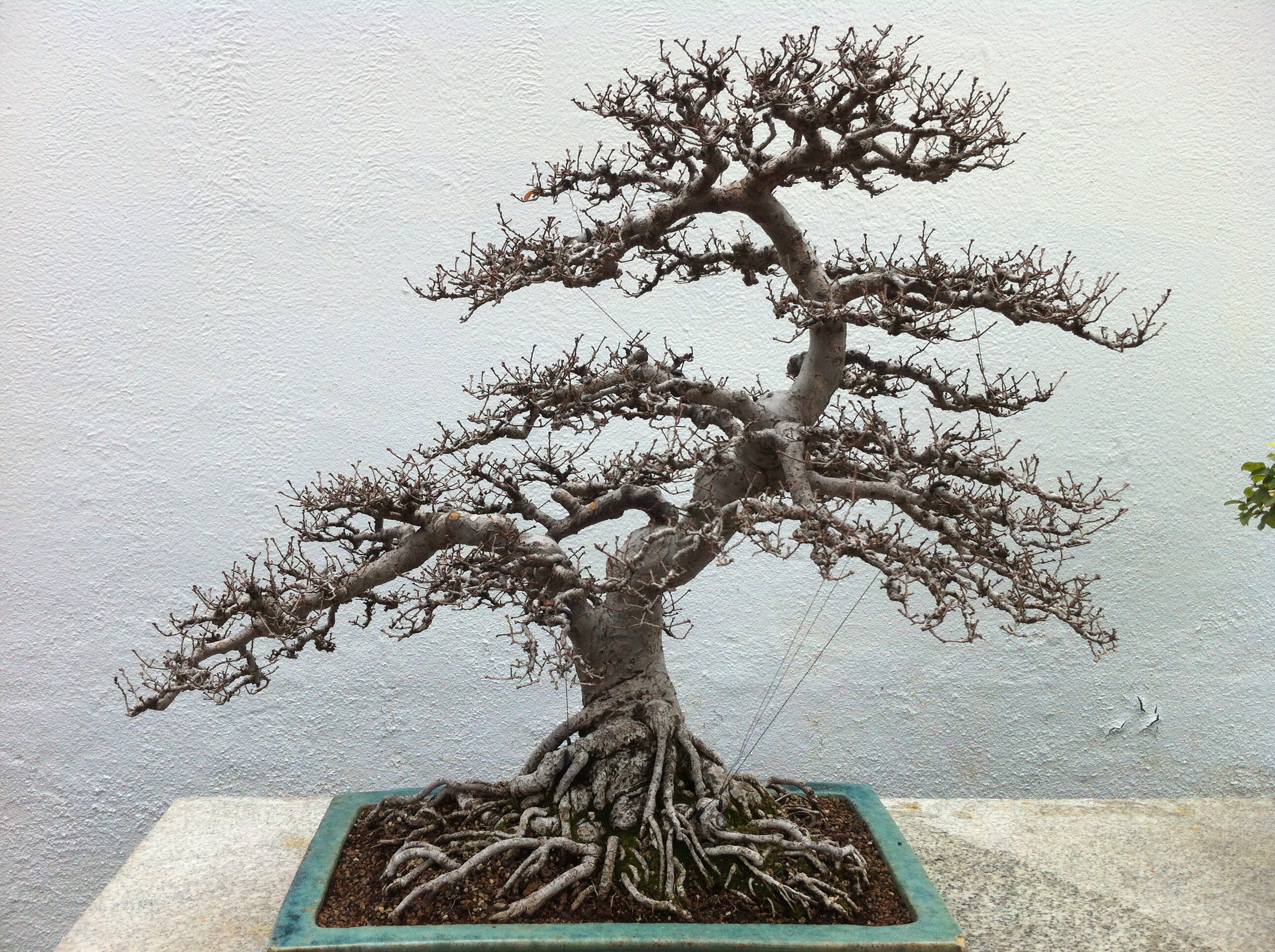
The alcohol dehydrogenase gene, (Adh), is an incredibly well studied enzyme, both from the perspective of its biochemical properties, but also as an early example of protein and genetic variation that was studied but many, many population geneticists. In the next few sections we’ll come back to this locus again and again.

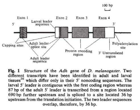
To orient us, I’ve taken Figure 1 directly from the now classic study DNA variation at Adh by Marty Kreitman (1983) shows the structure of the Adh protein coding gene. This is a pretty average gene in the drosophila genome– a few exons, separated by introns that are a few hundreds of bp long.


Fig. 1. Drosophila Adh gene structure, from Kreitman (1983)

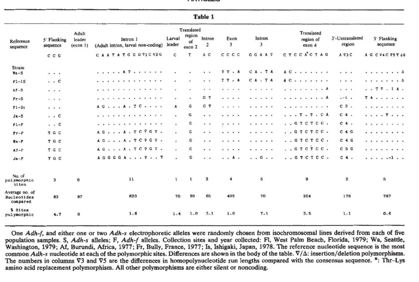
Kreitman, in what became a landmark study, described nucleotide variation in 11 strains of Drosophila melanogaster collected from a worldwide sample. In what more or less corresponds to all the “raw” data, take a look at the table of nucleotide variation shown in Figure 2. Here we see how sites vary according to their location in the gene structure. There are a few things to note:

there are variable positions in each part of the gene
there are more variable positions in introns than in exons on a percentage basis
some alleles (variant states) seem to be inherited together (more on linkage later)


Fig. 2. DNA polymorphism at Adh, from Kreitman (1983)

Loci, Alleles, and Identity¶

Before we go any further we need to get some nomenclature under our belts. The first distinction is that between locus and alleles. A locus is the chromosomal address where a DNA sequence lives. An allele is the version of that DNA sequence found at a locus. So we can talk about the Adh locus, the gene region on the chromosome, and we can talk about the alleles that we find at that locus (e.g., those shown in Figure 2). Most organisms are diploid, that is they contain two complete copies of the genome, one inherited from mom the other from dad. This means that any diploid individual may have two alleles at a locus, the maternal and paternal alleles.

Population genetics is concerned with describing patterns of allelic variation in natural populations of organism. Indeed for the population geneticist there are three ways that alleles might differ from each other:

By origin alleles may differ by origin in a generation if they come from the same locus on different chromosomes in the previous generation. For instance the alleles at a particular locus in a diploid individual differ by origin, because each was inherited from a distinct parental chromosome (mom and dad). Also if we consider the 11 Adh alleles shown above, those are different by origin.
By state alleles are said to be different by state if they, in someway, are different at the molecular level. For instance if we are looking at DNA sequences, two alleles are different by state if they have different sequences. These alleles could differ at a single nucleotide site or many, but either way they are said to differ by state. Moreover, we might not be considering DNA sequences at all. Alleles can vary by state if they are different lengths, or have different electrophoretic mobilities on a gel, or could be in reference to a specific position along a nucleotide or Amino Acid position. For instance, in Figure 2, there are (at least) two classes of alleles that differ by state, the Adh-f and Adh-s alleles which correspond to the fast vs slow allozyme polymorphism.
By descent allele differ by descent if they don’t share a common ancestor recently. In general all alleles at a locus are eventually descended from a common ancestor, so this definition is really only useful in thinking about shorter timescales, say fewer than 10 generations. Two alleles that differ by descent may or may not also differ by state.

Genotype and Allele Frequencies¶

To begin we need to understand some simple population genetic “bookkeeping.” Consider a locus with two alleles (alternative forms of the DNA sequence that “reside” at that locus, e.g., one from mother other from father). Now consider a population of N individuals (N=population size); this means that there are 2N alleles in the population. We can thus talk about genotype frequencies and allele frequencies. Let’s turn our attention to a hypothetical locus, the $A$ locus. We will first assume that there are two alleles segregating at the $A$ locus, $A_1$ and $A_2$. These could be two allozyme alleles (i.e. fast vs. slow) or two variant nucleotides at a polymorphic position in a genome (i.e. a SNP). Three genotypes are possible at the $A$ locus: two homozygous genotypes, $A_1A_1$ and $A_2A_2$, and one heterozygous genotype $A_1A_2$. We write the relative frequency of a genotype as $x_{ij}$ as this table shows:

Genotype:	$A_1A_1$	$A_1A_2$	$A_2A_2$
Relative Frequency:	$x_{11}$	$x_{12}$	$x_{22}$

As relative frequencies must add to one we have $$\begin{aligned} x_{11} + x_{12} + x_{22} = 1 \end{aligned}$$

The subscripting of the heterozygotes is of course arbitrary. Following my old advisor John Gillespie, we will take the convention of referring to the heterozygote as $x_{12}$ rather than $x_{21}$ – you can only use one subscripting convention if you want to keep things straight.

Often in population genetics we are interested in allele frequencies rather than genotype frequencies. The frequency of the $A_1$ allele in a population is simply

\[\begin{aligned} p = x_{11} + \frac{1}{2}x_{12}, \end{aligned}\]

and the frequency of the $A_2$ allele is

\[\begin{aligned} q = 1 - p = x_{22} + \frac{1}{2}x_{12}.\end{aligned}\]

There are two ways to think about $p$, the frequency of the $A_1$ allele. The first way is as the relative frequency of the $A_1$ allele among all of the (two) alleles at the $A$ locus in our population. This is simple enough to get one’s head around. The second way to think about $p$ is as the probability that an allele picked by random from the population is the $A_1$ allele. Picking an allele at random is actually composed of two parts, 1) picking a genotype at random from the population and 2) then picking an allele from that genotype at random. With our three genotypes at the $A$ locus we could write down $p$ as

\[\begin{aligned} p = (x_{11}\times1) + (x_{12}\times\frac{1}{2}) + (x_{22}\times0).\end{aligned}\]

This expression for $p$ is broken down into three terms which reveal the three mutually exclusive ways to sample an $A_1$ allele from the population and their associated probabilities. Let’s consider the first term in this sum. This represents the joint event where we sample an $A_1A_1$ individual from our population (this occurs with probability $x_{11}$) and then sample an $A_1$ allele from that individual (this occurs with probability one). In the second term we consider the joint event of sampling an $A_1A_2$ individual (with probability $x_{12}$) and then sampling an $A_1$ allele (with probability $\frac{1}{2}$). Now ask yourself, what is that zero doing in the third term?? Got it?

Let’s use a concrete example to drive this all home. Consider a population of $N = 100$ individuals. We observe the following number of genotypes at our $A$ locus:

Genotype:	$A_1A_1$	$A_1A_2$	$A_2A_2$
Observed Numbers:	25	50	25
Relative Frequencies:	0.25	0.50	0.25

The relative genotypic frequencies, the $x_{ij}s$, are simple to calculate, just divide the number of each observed genotype by the population size. For example, $x_{12} = \frac{50}{100} = 0.5$. Now let’s calculate allele frequencies. The allele frequency of the $A_1$ allele, $p$, is found in the following way

\[\begin{aligned} p = (0.25 \times 1) + (0.5 \times\frac{1}{2}) + (0.25\times0) = 0.5. \end{aligned}\]

So in this trivial example $p = q = 0.5$.

Let’s do a slightly less contrived example. Consider the following table of genotypes taken from screening African school children for the sickle cell anemia locus. In this case recall that $A_1A_1$ individuals are healthy, $A_2A_2$ individuals are sick, and heterozygotes show increased resistance to malaria.

Genotype:	$A_1A_1$	$A_1A_2$	$A_2A_2$
Observed Numbers:	411	1404	185
Relative Frequencies:	0.2055	0.702	0.0925

First double check that I have gotten relative genotypic frequencies correct. Next calculate the allele frequencies. I get $p = 0.556$, what do you get?

The Hardy-Weinberg Law¶

Perhaps the best known population genetic model is the famous Hardy-Weinberg law, which describes the relationship between allele and genotype frequencies at an autosomal locus in an equilibrium randomly mating population. By equilibrium we mean a population that is not undergoing evolutionary forces such as selection, mutation, or genetic drift. By randomly mating we mean that individuals mate with each other irrespective of relatedness or geography. Populations where cousins mate are not randomly mating- this is called inbreeding. Populations where $A_1A_1$ individuals are more likely to mate with other $A_1A_1$ individuals are not randomly mating- we call this assortative mating. Similarly if one is more likely to mate with their neighbors, geographically, than this too is not random mating.

The easiest way to envision an honest to goodness Hardy-Weinberg population is as hermaphrodite, broadcast spawners, something like sponges or corals. Individuals produce both sperm and eggs, and randomly let them go into the environment to meet up and form zygotes. In this way the probability of forming an $A_1A_1$ zygote is the product of the probability of choosing an $A_1$ egg, $p$, and the probability of choosing an $A_1$ sperm (these probabilities are identical because of our assumption of hermaphrodites). Thus the probability of randomly forming an $A_1A_1$ zygote is $p^2$. By similar reasoning, the probability of forming an $A_2A_2$ zygote is $q^2$. There are two ways to form an $A_1A_2$ heterozygote. The first way is with an $A_1$ sperm and an $A_2$ egg. This probability is $pq$. The second way would be with an $A_2$ sperm and an $A_1$ egg. Again, this probability is $pq$. Because we sum mutually exclusive probabilities, the total probability of randomly forming a heterozygote is $2pq$. Congratulations, you’ve just derived your first population genetic model.

After one round of random mating the frequencies of the three genotypes at our locus are

Genotype:	$A_1A_1$	$A_1A_2$	$A_2A_2$
H-W Frequency:	$p^2$	$2pq$	$q^2$

These are the Hardy-Weinberg genotype frequencies. They only depend on allele frequencies, thus if you know $p$ you know all of the genotype frequencies.

A couple of things to note about random mating in our diploid hermaphrodites:

Allele frequencies are unaffected by random mating. Random mating can change genotype frequencies, but not allele frequencies, thus after one round of mating Hardy-Weinberg genotype frequencies will remain unchanged, forever!
In our diploid hermaphrodites it only takes one generation to achieve H-W equilibrium proportions. In species with separate sexes it takes two generations.
To come up with genotype frequencies after random mating we only need to know allele frequencies before random mating, not genotype frequencies.

Let’s step back to our numerical example from human sickle cell anemia. Our goal will be to predict Hardy-Weinberg expected values for genotype frequencies at this locus, given our observed allele frequencies. We have already done the first step which is to calculate the frequency of the $A_1$ allele, in this case $p = 0.556$. Now lets calculate the frequency of the $A_2$ allele, $q = 1 - p = 1 - 0.556 = 0.444$. Using these allele frequencies we can fill out a table of genotype frequencies

Genotype:	$A_1A_1$	$A_1A_2$	$A_2A_2$
H-W Frequency:	$p^2$	$2pq$	$q^2$
H-W Expected Frequencies:	0.309	0.494	0.197
Observed Frequencies:	0.2055	0.702	0.0925

Compare the observed genotypic frequencies with what we would expect from the Hardy-Weinberg law. Pretty different, huh? In particular I want you to notice how we observe many more heterozygotes than we would expect. This is what is called in the business an excess of heterozygotes. Why are we seeing this difference? Which of our Hardy-Weinberg assumptions have failed us? One can always test for a significant deviation from our H-W expectation using a chi-square statistic.

So what happens in species with separate sexes (dioecious species)? What if genotype frequencies are different between the sexes? At the most extreme, lets imagine that all males are $A_1A_1$ and all females are $A_2A_2$. With an equal sex ratio the frequency of the $A_1$ allele is $p=0.5$. In this case, after one round of random mating every individual in the population is $A_1A_2$, and the frequencies of the heterozygotes is one. This is clearly far from the Hardy-Weinberg expected genotype frequencies. However, after just one more round of random mating the frequencies of the $A_1A_1$, $A_1A_2$, and $A_2A_2$ genotypes are returned to their Hardy-Weinberg values of $\frac{1}{4},\frac{1}{2}$, and $\frac{1}{4}$. So even for dioecious species with very different allele frequencies it only takes two rounds of random mating to get back our H-W expected genotype frequencies.

Heterozygosity¶

As we talked about in the last lecture, getting a handle on the amounts of genetic variation within a population is very important both to genetics and evolutionary theory. One broad way to describe the “amount” of variation that exists at the genetic level is to describe a population by the probability of sampling a heterozygous genotype from it. For obvious reasons we call this measure the heterozygosity of a population.

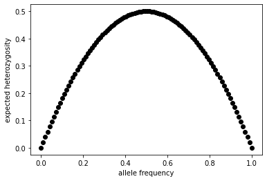
Our cursory look at the Hardy-Weinberg law suggests that heterozygosity might depend on allele frequencies. Figure 1 shows a plot of the frequency of heterozygotes as a function of the $A_1$ allele frequency under Hardy-Weinberg conditions. Ask yourself this simple question- at what allele frequency is the probability of sampling a heterozygote from a population maximized? Does this make intuitive sense to you?

import numpy as np
import matplotlib.pyplot as plt

def het(p):
    """
    Calculate the expected heterozygosity of a population
    from the allele frequency, p
    """
    return np.array(2 * p * (1 - p))

allele_freqs = np.linspace(0,1,100)
expected_het = het(allele_freqs)
plt.scatter(allele_freqs, expected_het, label="expected heterozygosity", c="black")

plt.xlabel("allele frequency")
plt.ylabel("expected heterozygosity")

Text(0, 0.5, 'expected heterozygosity')

Before moving on to a formal treatment of heterozygosity, let’s first generalize the Hardy-Weinberg law to the case where we have more than two alleles at a locus. Good examples of such loci in actual genomes would include microsatellites or allozyme polymorphisms, as opposed to SNPs which tend to be diallelic. If we have $k$ alleles at a locus, $A_i$, $i=1...k$, let their frequencies be called $p_i$, $i=1...k$. It follows that the frequency of the $A_iA_i$ homozygote after random mating should be $p_{i}^2$ and the frequency of the $A_iA_j$ heterozygote should be $2p_ip_j$. Simple enough, but make sure this is straight in your head. It might be helpful to write out the three allele example in its entirety at this point. Moving on, the total frequency of homozygotes in our population is

\[\begin{aligned} G = \sum_{i=i}^{k}p_{i}^2. \end{aligned}\]

$G$ here is called the homozygosity of a locus. Ask yourself- what is the probabilistic interpretation of $G$? The heterozygosity of a locus is the complement (in probability space) of homozygosity

\[\begin{aligned} H = 1 - G = 1 - \sum_{i=i}^{k}p_{i}^2. \end{aligned}\]

For populations that obey the assumptions of the Hardy-Weinberg law, heterozygosity will actually equal the frequency of heterozygotes, however heterozygosity is calculated using only allele frequencies. Because of this heterozygosity is often used to describe populations that don’t conform to H-W assumptions. In many ways it’s just a convenient measure- like temperature.

Simulating Hardy-Weinberg Expectations¶

Next let’s use SLiM to simulate a finite population that is randomly mating. We will add a single mutation to our population at the beginning at a specific frequency, $p_0$, and then watch how the genotype frequencies change over time.

%load_ext slim_magic

import pandas as pd
import numpy as np
from matplotlib import pyplot as plt
from IPython.display import display, SVG

%%slim_stats_reps_rstack 10 --out df
// set up a single locus simulation of drift
initialize()
{
    // set the overall mutation rate
    // no mutation in this simulation
    initializeMutationRate(0);
    // m1 mutation type: neutral
    initializeMutationType("m1", 0.5, "f", 0.0);
    // single locus simulation
    // g1 genomic element type: uses m1 probability 1
    initializeGenomicElementType("g1", c(m1), c(1.0));
    // uniform chromosome of length 1 site
    initializeGenomicElement(g1, 0, 0);
    // uniform recombination along the chromosome
    initializeRecombinationRate(0);
    suppressWarnings(T);
}

// create a population of 100 individuals
1 {
    sim.addSubpop("p1", 100);
    // sample 100 haploid genomes 
    target = sample(p1.genomes, 100);
    // add a mutation to those genomes
    // H_0 = 0.5 here
    target.addNewMutation(m1,0, 0);
    cat("generation,p,x11,x12,x22\\n");
}
1:300 late(){
    inds = p1.sampleIndividuals(100);
    // record the number of mutations in each individual
    ind_count = inds.countOfMutationsOfType(m1);
    counts = c(0, 0, 0);
    for (x in ind_count)
        counts[x] = counts[x] + 1;
    // divide by popn size to get genotype freqs
    counts = counts / 100;
    // allele freq of A_1 allele in current gen
    freqs = sim.mutationFrequencies(p1);
    // each gen print out the gen, the allele freqs, and the counts
    if (length(freqs) > 0.0)
        catn(sim.generation + "," + freqs + "," + paste(counts, sep=","));
    }
// run to generation 0
300 late() {
    sim.simulationFinished();
    }

Next let’s write a tiny function that will take an allele frequency and return the expected HW genotype frequencies

def hwe(p):
    return np.array([p**2, 2 * p * (1 - p), (1 - p)**2])

#run that function for 100 pts between (0,1)
expected = hwe(np.linspace(0,1,100))

Finally let’s plot for our simulations how the observed genotype frequencies compare to that expected, given the observed allele frequency

#plot simulated
plt.scatter(df.p, df.x11, label="A_11 frequency")
plt.scatter(df.p, df.x12, label="A_12 frequency")
plt.scatter(df.p, df.x22, label="A_22 frequency")


#plot expected
plt.plot(np.linspace(0,1,100),expected[0,:], c="red", linestyle="dotted", label="HWE expected")
plt.plot(np.linspace(0,1,100),expected[1,:], c="red", linestyle="dotted")
plt.plot(np.linspace(0,1,100),expected[2,:], c="red", linestyle="dotted")

plt.legend()
plt.xlabel("allele frequency")
plt.ylabel("genotype frequency")

Text(0, 0.5, 'genotype frequency')

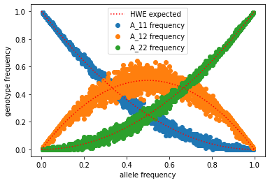
Wow an awesome fit! Why does this look so good?

Welcome to Population Genetics

Natural Selection

Bio 610-- Intro to Population Genetics