Migration and Gene Flow
Contents
Migration and Gene Flow
In population genetics, the term “migration” is really meant to describe Gene flow, defined as the movement of alleles from one area (deme, population, region) to another. Gene flow assumes some form of dispersal or migration (wind pollination, seed dispersal, birds flying, etc.) but dispersal is not gene flow (genes must be transferred, not just their carriers)
We are going to build a model of gene flow in exactly the same way we studied mutation. Consider two populations, a mainland population and an island population. Each of these populations has the \(A_1\) allele at frequencies \(p_{main}\) and \(p_{island}\) respectively. Assume that gene flow is one way, from mainland to island and that the proportion of individuals who become parents in the island population is \(m\). Although I’ve said this is a proportion, also notice that we could consider this a probability interchangeably. After a round of migration, in the island population there are then two sources for alleles, they could be from the island population originally with probability \(1-m\), or they could have migrated from the mainland with probability \(m\). This means that after migration the allele frequency of \(A_1\) in the island population is $\(\begin{aligned} p_{island}' = p_{island}(1-m) + p_{main}m. \end{aligned}\)$
Simple enough right? Now lets to what comes naturally and study the change in allele frequency as a result of mutation. Following what we have done in our other analyses,
Beautiful. Now we have a very simple expression for how allele frequencies in the island population should change due to gene flow from the mainland population. This change in allele frequency makes sense- it only depends on the amount of migration and the differences in allele frequencies between the two populations. It’s simple enough to generalize this to multiple populations, or to populations at different distances away from one another.
Let’s plot \(\Delta_{m}p_{island}\)
%load_ext slim_magic

import pandas as pd
import numpy as np
from matplotlib import pyplot as plt
from IPython.display import display, SVG
def delta_m(p_m, p_i, m):
    return m * (p_m - p_i)

x = np.linspace(0, 1, 100)
p_m = 0.5
p_i = 0.5
plt.plot(x, delta_m(x, p_m, p_i))
plt.vlines(p_i,-0.3, 0.3, linestyles='dashed')
plt.ylabel('$\Delta m$')
plt.xlabel('$p_m$')
Text(0.5, 0, '$p_m$')
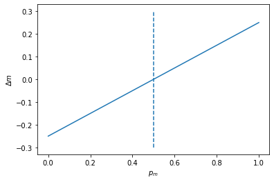
the dotted line here represents the frequency of the island population. Ask yourself, why does \(\Delta_{m}p_{island} = 0\) at that point?
Non-random mating
When individuals do not mate randomly, the assumptions of the Hardy-Weinberg law are no longer met. A potent force that leads to non-random mating is population subdivision, where for instance individuals in certain parts of the range are more likely to mate with one another than they are with individuals that are far away or in a separate patch connected via migration.
Let’s motivate this with an example simulation from SLiM, that’s a spin on one we looked at on the first day.
%%slim_stats_reps_rstack 10 --out subdivision
// set up a single locus simulation of drift
initialize()
{
    // set the overall mutation rate
    initializeMutationRate(0);
    // m1 mutation type: neutral
    initializeMutationType("m1", 0.5, "f", 0.0);
    // g1 genomic element type: uses m1 probability 1
    initializeGenomicElementType("g1", c(m1), c(1.0));
    // uniform chromosome of length 1 site
    initializeGenomicElement(g1, 0, 0);
    // uniform recombination along the chromosome
    initializeRecombinationRate(0);
    suppressWarnings(T);
}

// create 2 populations of 50 individuals
1 {
    sim.addSubpop("p1", 50);
    sim.addSubpop("p2", 50);
    // sample 50 haploid genomes from the first population
    target = sample(p1.genomes, 50);
    // add a mutation to those genomes
    target.addNewMutation(m1,0, 0);
    //print header for the output
    cat("generation,p,x11,x12,x22\\n");
}
1:300 late(){
    inds1 = p1.sampleIndividuals(50);
    inds2 = p2.sampleIndividuals(50);
    inds = c(inds1, inds2);
    ind_count = inds.countOfMutationsOfType(m1);
    counts = c(0, 0, 0);
    for (x in ind_count)
        counts[x] = counts[x] + 1;
    counts = counts / 100;
    freqs1 = sim.mutationFrequencies(p1);
    freqs2 = sim.mutationFrequencies(p2);
    freqs = freqs1 + freqs2;
    if (length(freqs) > 0.0)
        catn(sim.generation + "," + freqs + "," + paste(counts, sep=","));
    }
// run to generation 0
300 late() {
    sim.simulationFinished();
    }
def hwe(p):
    return np.array([p**2, 2 * p * (1 - p), (1 - p)**2])

#run that function for 100 pts between (0,1)
expected = hwe(np.linspace(0,1,100))

#plot simulated
plt.scatter(subdivision.p, subdivision.x11, label="A_11 frequency")
plt.scatter(subdivision.p, subdivision.x12, label="A_12 frequency")
plt.scatter(subdivision.p, subdivision.x22, label="A_22 frequency")


#plot expected
plt.plot(np.linspace(0,1,100),expected[0,:], c="red", linestyle="dotted", label="HWE expected")
plt.plot(np.linspace(0,1,100),expected[1,:], c="red", linestyle="dotted")
plt.plot(np.linspace(0,1,100),expected[2,:], c="red", linestyle="dotted")

plt.legend()
plt.xlabel("allele frequency")
plt.ylabel("genotype frequency")
Text(0, 0.5, 'genotype frequency')
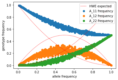
So we can see in this example of two, subdivided populations which don’t share migrants that we are deviating sharply from our Hardy Weinberg expectations. In this specific case you might notice that there are too few heterozygotes relative to our expectations from Hardy Weinberg. Let’s model this.
Generalized Hardy-Weinberg
Genotype: |
\(A_1A_1\) |
\(A_1A_2\) |
\(A_2A_2\) |
|---|---|---|---|
H-W Frequency: |
\(p^2(1-F) + pF\) |
\(2pq(1-F)\) |
\(q^2(1-F) + qF\) |
We’ve introduced a new variable here, \(F\), which the deviations from the expected frequencies. If \(F=0\) we are back to our expected HW values. If \(0 < F \leq 1\) then there is an excess of homozygotes relative to expectations, if \(F < 0\) there is an excess of heterozygotes.
Next lets look a bit more closely at a flavor of \(F\) that we use in the particular case of subdivision that we are simulating above. Let’s call that \(Fst\). Next imagine a species arranged as above in two discrete subpopulations that we could call subpop1 and subpop2. Next let’s imagine that the current allele and genotype frequencies in each of my subpops is as follows:
Genotype: |
\(A_1\) |
\(A_1A_1\) |
\(A_1A_2\) |
\(A_2A_2\) |
|---|---|---|---|---|
Subpop1 Frequency: |
0.25 |
0.0625 |
0.375 |
0.5625 |
Subpop2 Frequency: |
0.75 |
0.5625 |
0.375 |
0.0625 |
Species-wide Frequency: |
0.5 |
0.3125 |
0.375 |
0.3125 |
HWE Frequency: |
0.5 |
0.25 |
0.5 |
0.25 |
here is species-wide frequency is simple the average of the two subpopulations, assuming they are of equal size. Here, even though each subpopulation has HW expected proportions of genotype frequencies, the species as a whole does not. In fact there are too few heterozygotes relative to our expectations. Let’s measure this with \(Fst\), we say
In general, populations that have insufficient migration between them to homogenize allele frequencies across the landscape with show positive \(F_{st}\) like this in pooled samples. This deficiency of heterozygotes in cryptically sampled subpopulations is sometimes called the Wahlund effect.
SLiM simulations with migration
Okay let’s modify our simulations above to include migration between populations. Let’s start with little migration and then increase it back in.
%%slim_stats_reps_rstack 10 --out subdivision
// set up a single locus simulation of drift
initialize()
{
    // set the overall mutation rate
    initializeMutationRate(0);
    // m1 mutation type: neutral
    initializeMutationType("m1", 0.5, "f", 0.0);
    // g1 genomic element type: uses m1 probability 1
    initializeGenomicElementType("g1", c(m1), c(1.0));
    // uniform chromosome of length 1 site
    initializeGenomicElement(g1, 0, 0);
    // uniform recombination along the chromosome
    initializeRecombinationRate(0);
    suppressWarnings(T);
}

// create 2 populations of 50 individuals
1 {
    sim.addSubpop("p1", 50);
    sim.addSubpop("p2", 50);
    // add migration between the two populations
    p1.setMigrationRates(p2, 0.001);
    p2.setMigrationRates(p1, 0.001);

    // sample 50 haploid genomes from the first population
    target = sample(p1.genomes, 50);
    // add a mutation to those genomes
    target.addNewMutation(m1,0, 0);
    //print header for the output
    cat("generation,p,x11,x12,x22\\n");
}
1:300 late(){
    inds1 = p1.sampleIndividuals(50);
    inds2 = p2.sampleIndividuals(50);
    inds = c(inds1, inds2);
    ind_count = inds.countOfMutationsOfType(m1);
    counts = c(0, 0, 0);
    for (x in ind_count)
        counts[x] = counts[x] + 1;
    counts = counts / 100;
    freqs1 = sim.mutationFrequencies(p1);
    freqs2 = sim.mutationFrequencies(p2);
    freqs = (freqs1 + freqs2) / 2;
    if (length(freqs) > 0.0)
        catn(sim.generation + "," + freqs + "," + paste(counts, sep=","));
    }
// run to generation 0
300 late() {
    sim.simulationFinished();
    }
#plot simulated
plt.scatter(subdivision.p, subdivision.x11, label="A_11 frequency")
plt.scatter(subdivision.p, subdivision.x12, label="A_12 frequency")
plt.scatter(subdivision.p, subdivision.x22, label="A_22 frequency")


#plot expected
plt.plot(np.linspace(0,1,100),expected[0,:], c="red", linestyle="dotted", label="HWE expected")
plt.plot(np.linspace(0,1,100),expected[1,:], c="red", linestyle="dotted")
plt.plot(np.linspace(0,1,100),expected[2,:], c="red", linestyle="dotted")

plt.legend()
plt.xlabel("allele frequency")
plt.ylabel("genotype frequency")
Text(0, 0.5, 'genotype frequency')
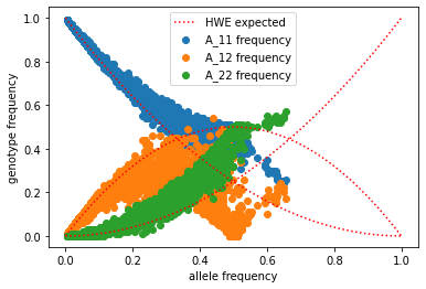
what do you notice here? what is the pattern?