Deep Operator Network

Deep Operator Networks (DeepONets) learn the operator that maps a set of functions to another function. Using the same PDE as the PINN and P\(^2\)INN examples, we will learn the mapping \(G: \{N(t), g_0(x)\} \rightarrow g(x,t)\), where \(N(t)\) is the relative population size change and \(g_0\) is the initial condition of the PDE. Our model's coordinate inputs will be \((x,t)\), as before, and the auxiliary inputs will be arrays of \(N(t)\) and \(g_0(x)\) evaluated at fixed \(t_s\) and \(x_s\) sensor points.

As before, we will enforce \(N(t = 0) = 1\) and choose a linear population size change function, \(N(t| N_s) = N_s t + 1\). We will evaluate \(N(t| N_s)\) for different \(N_s\) values and across a fixed set of sensor points \(t_s\). The resulting array will have a shape (NUM_NS_PTS, NUM_TS_PTS).

Because \(N(t = 0) = 1\), the initial condtion

\[ g_0(x) = \theta\frac{1 - e^{-2\gamma(1-x)}}{1 - e^{-2\gamma}} \]

only depends on \(\gamma\), so we can construct our training data by varying \(\gamma\) and evaluating \(g_0(x| \gamma)\) across a fixed set of sensor points \(x_s\). The resulting data array will have a shape (NUM_G_PTS, NUM_XS_PTS).

import os

os.environ["CUDA_VISIBLE_DEVICES"] = "1,2"

import jax

jax.config.update("jax_enable_x64", True)

import equinox as eqx
import jax.numpy as jnp
import jax.random as jr
import matplotlib.pyplot as plt
from jaxtyping import Array

from popinn import AdamConfig, LBFGSConfig, Loss, ResidualTerm, plot_training_history, train_model, warmup_cosine

# Fixed values

THETA = 1.0  # population-scaled mutation rate
NFUNC = lambda t, N_s: N_s * t + 1.0  # linear population size increase

# gamma bounds
GMIN = 0.01
GMAX = 5.0

# gamma grid length
NUM_G_PTS = 30
NUM_XS_PTS = 31

# N_s bounds:
NS_MIN = 1.0
NS_MAX = 10.0

# N_s grid length
NUM_NS_PTS = 30
NUM_TS_PTS = 30

# x-coordinate bounds
XMIN = 0.0
XMAX = 1.0

# t-coordinate maximum
TMAX = 1.0

# colocation grid lengths
NUM_PDE_PTS = 30  # points per spatial/temporal coordinate axis on PDE interior
NUM_EDGE_PTS = 256  # points used to sample the IC/boundary coordinate lines

Residual Terms

In this example, \(N(t|N_s)\) and \(g_0(x| \gamma)\) are the auxiliary inputs of our model. Like in the P\(^2\)INN example, there are residual equations that will also need the value of \(\gamma\) and/or \(N_s\), e.g. the PDE:

\[ \frac{\partial g}{\partial t} = \frac{1}{2N(t|N_s)}x (1 - x)\frac{\partial^2 g}{\partial x^2}- \gamma x (1 - x)\frac{\partial g}{\partial x}. \]

We therefore must pass \(\gamma\) and \(N_s\) through the aux argument of our residual functions, but only pass \(N(t|N_s)\) and \(g_0(x| \gamma)\) as the aux argument of the model. Since we'll be unpacking aux for each residual term, we'll define a convenience function to do it for us:

def unpack(aux):
    (Nvals_, Ns_), (ics_, gamma_) = aux
    return (Nvals_, ics_), Ns_, gamma_  # group the model inputs together in a tuple

We'll wait until the Training Data section to explain how to structure aux. For now, note that Nvals_ and ics_ in the above function will each be a 1D array of \(N(t|N_s)\) and \(g_0(x|\gamma)\) values evaluated at a set of \(t_s\) and \(x_s\) points for a fixed value of \(N_s\) and \(\gamma\).

# PDE residual
def pde_residual(model):
    def r(x, t, aux):
        model_aux, Ns, gamma = unpack(aux)  # separate out model aux inputs

        dg_dx = model.D(0)(x, t, model_aux)  # d/dx
        dg_dt = model.D(1)(x, t, model_aux)  # d/dt
        d2g_dx2 = model.D(0, 0)(x, t, model_aux)  # d2/dx2

        diff = x * (1.0 - x) / (2.0 * NFUNC(t, Ns)) * d2g_dx2  # diffusion
        sel = gamma * x * (1.0 - x) * dg_dx  # selection

        # we weight the per-point residuals by their frequency x, as the gradients
        # tend to be very large at low-frequency. Wrapping x in
        # jax.lax.stop_gradient treats it like a constant, rather than a differentiable
        # quantity, so it doesn't change the PDE we are trying to learn
        return (dg_dt + sel - diff) * jax.lax.stop_gradient(x)

    return r

# Left BC residual
def left_bc_residual(model):
    def r(x, t, aux):
        model_aux, Ns, gamma = unpack(aux)
        return model(x, t, model_aux) - THETA * NFUNC(t, Ns)

    return r

# Right BC residual
def right_bc_residual(model):
    def r(x, t, aux):
        model_aux, Ns, gamma = unpack(aux)
        return model(x, t, model_aux)

    return r

def initial_g(x, _gamma):
    neutral = 1.0 - x
    selected = jnp.expm1(-2.0 * _gamma * (1.0 - x)) / jnp.expm1(-2.0 * _gamma)
    # jnp.where keeps this differentiable and vmap-friendly across gamma.
    return THETA * jnp.where(jnp.greater(jnp.abs(_gamma), 1e-5), selected, neutral)


# initial condition residual
def ic_residual(model):
    def r(x, t, aux):
        model_aux, Ns, gamma = unpack(aux)
        return model(x, t, model_aux) - initial_g(x, gamma)

    return r

The Loss initialization stays the same:

total_loss = Loss(
    [
        ResidualTerm(name="pde", residual_fn=pde_residual),
        ResidualTerm(name="left_bc", residual_fn=left_bc_residual),
        ResidualTerm(name="right_bc", residual_fn=right_bc_residual),
        ResidualTerm(name="ic", residual_fn=ic_residual),
    ]
)

Training Data

Now we need to evaluate the input functions for different parameter values and across fixed sensor points. We'll use a function that gives us exponentially spaced data for the interior PDE collocation points and sensor points.

def exponential_grid(pts, crwd=8, where="both"):
    """
    This function was adapted from `exponential_grid` in the dadi package (https://github.com/RyanGutenkunst/dadi/blob/32d6a6003675a7b015149f3e04d06bafe3908de1/dadi/Numerics.py#L215-L231).
    - An exponentially spaced grid.
    - crwd controls the degree to which grid points crowd against x=0 or x=1.
    - where: 'both' or 'left' or 'right'

    """
    if where == "both":
        xlim = (-1.0, 1.0)
    elif where == "left":
        xlim = (-1.0, 0.0)
    elif where == "right":
        xlim = (0.0, 1)
    else:
        raise ValueError("`where` argument can be 'both', 'left', or 'right'.")
    unif = jnp.linspace(*xlim, pts + 1)
    grid = 1.0 / (1.0 + jnp.exp(-crwd * unif))

    # Normalize
    grid = (grid - grid[0]) / (grid[-1] - grid[0])
    return grid[1:]

class TrainingData(eqx.Module):
    pde_coords: tuple[Array]
    ic_coords: tuple[Array]
    left_bc_coords: tuple[Array]
    right_bc_coords: tuple[Array]
    aux: tuple


X_pde = exponential_grid(NUM_PDE_PTS, crwd=2.0, where="left")
T_pde = jnp.linspace(0, TMAX, NUM_PDE_PTS)

X_ic = jnp.linspace(XMIN, XMAX, NUM_EDGE_PTS)
T_ic = jnp.zeros(1)

T_bc = jnp.linspace(0, TMAX, NUM_EDGE_PTS)
X_lbc = XMIN * jnp.ones(1)
X_rbc = XMAX * jnp.ones(1)

# all of the above code is the same as P2INN
# Get the N(t) array
TS = jnp.linspace(0, TMAX, NUM_TS_PTS)
NS = jnp.linspace(NS_MIN, NS_MAX, NUM_NS_PTS)
NVALS = jax.vmap(NFUNC, in_axes=(None, 0))(TS, NS)  # map over the set of Ns values
assert NVALS.shape == (NUM_NS_PTS, NUM_TS_PTS)

# Get the g_0(x) array
XS = exponential_grid(NUM_XS_PTS, crwd=2.0, where="left")
GAMMA = jnp.linspace(GMIN, GMAX, NUM_G_PTS)
ICVALS = jax.vmap(initial_g, in_axes=(None, 0))(XS, GAMMA)  # map over the set of gamma values
assert ICVALS.shape == (NUM_G_PTS, NUM_XS_PTS)

data = TrainingData(
    pde_coords=(X_pde, T_pde),
    ic_coords=(X_ic, T_ic),
    left_bc_coords=(X_lbc, T_bc),
    right_bc_coords=(X_rbc, T_bc),
    aux=((NVALS, NS), (ICVALS, GAMMA)),  # construct the aux tuple, packaging correlated quantities that share their 0th axis in their own tuple
)

Important syntax note

The the grid evaluation method used by ResidualTerm expects aux to be packaged in a specific way in order to properly broadcast the training data over the per-point residual function.

In this example, the proper packaging is

aux = ((NVALS, NS), (ICVALS, GAMMA))

Notice that 1D NS array was used to calculate the 2D NVALS array and their 0th axis has the same length. The same goes for GAMMA and ICVALS. Even though the model's auxiliary inputs are only NVALS and ICVALS, the residual functions we defined above require NS and GAMMA as additional auxiliary inputs. To ensure the individual parameter values are passed to the residual function alongside their corresponding function values, we can package them together in a tuple in aux. This will signal to eval_grid that it should zip their shared 0th axis during the cartesian product. For example, the PDE residual output will have the shape (NUM_G_PTS, NUM_NS_PTS, NUM_PDE_PTS, NUM_PDE_PTS) before it applies the metric to reduce it to a scalar.

The grid axis should always be the 0th axis of each array; all trailing axes are assumed to be per-point inputs. This is why we included the assertions above that check ICVALS.shape == (NUM_G_PTS, NUM_XS_PTS) and NVALS.shape == (NUM_NS_PTS, NUM_TS_PTS).

Initialize Model and Train

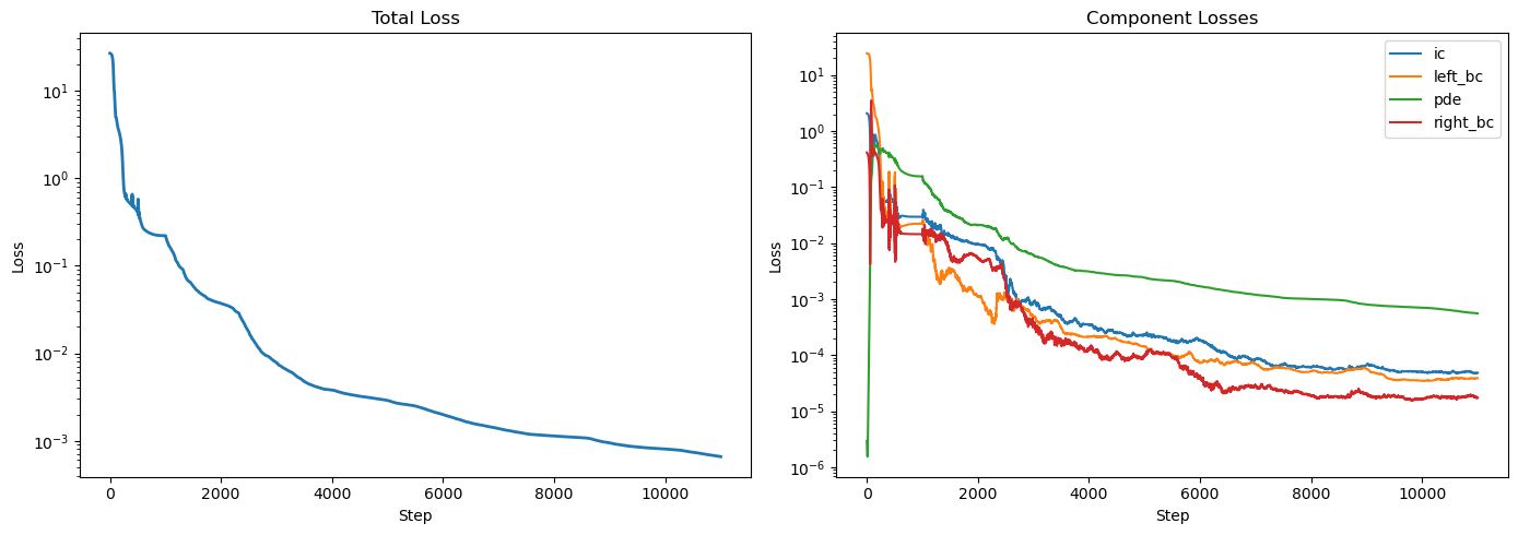
We'll first train with 1000 Adam steps, then 10k of L-BFGS:

key = jr.PRNGKey(3)
from popinn import DeepONet

model = DeepONet(key, branch_input_dim=(NUM_TS_PTS, NUM_XS_PTS), trunk_input_dim=2, branch_depth=(4, 4), trunk_depth=2)


model, history = train_model(
    model,
    data,
    total_loss,
    [AdamConfig(log_every=500, num_epochs=1000, lr=warmup_cosine(peak_lr=5e-4, num_epochs=1000)), LBFGSConfig(log_every=500, num_epochs=10000)],
)

[Adam] Starting (1000 epochs)
[Adam] Epoch      1 | total: 2.68e+01 | ic: 2.07e+00  left_bc: 2.43e+01  pde: 2.94e-06  right_bc: 4.12e-01
[Adam] Epoch    500 | total: 4.08e-01 | ic: 5.29e-02  left_bc: 3.01e-02  pde: 3.06e-01  right_bc: 1.89e-02
[Adam] Epoch   1000 | total: 2.21e-01 | ic: 2.94e-02  left_bc: 2.21e-02  pde: 1.55e-01  right_bc: 1.44e-02
[L-BFGS] Starting (10000 max iterations)
[L-BFGS] Step      1 | total: 2.21e-01 | ic: 2.89e-02  left_bc: 2.19e-02  pde: 1.56e-01  right_bc: 1.36e-02
[L-BFGS] Step    500 | total: 5.89e-02 | ic: 1.35e-02  left_bc: 3.22e-03  pde: 3.62e-02  right_bc: 6.03e-03
[L-BFGS] Step   1000 | total: 3.71e-02 | ic: 9.63e-03  left_bc: 1.11e-03  pde: 2.10e-02  right_bc: 5.34e-03
[L-BFGS] Step   1500 | total: 1.77e-02 | ic: 2.61e-03  left_bc: 1.08e-03  pde: 1.22e-02  right_bc: 1.74e-03
[L-BFGS] Step   2000 | total: 7.75e-03 | ic: 8.86e-04  left_bc: 4.79e-04  pde: 6.05e-03  right_bc: 3.37e-04
[L-BFGS] Step   2500 | total: 4.77e-03 | ic: 5.12e-04  left_bc: 3.06e-04  pde: 3.79e-03  right_bc: 1.64e-04
[L-BFGS] Step   3000 | total: 3.80e-03 | ic: 3.46e-04  left_bc: 2.13e-04  pde: 3.12e-03  right_bc: 1.28e-04
[L-BFGS] Step   3500 | total: 3.23e-03 | ic: 2.56e-04  left_bc: 1.92e-04  pde: 2.66e-03  right_bc: 1.15e-04
[L-BFGS] Step   4000 | total: 2.89e-03 | ic: 2.25e-04  left_bc: 1.44e-04  pde: 2.42e-03  right_bc: 9.81e-05
[L-BFGS] Step   4500 | total: 2.49e-03 | ic: 1.76e-04  left_bc: 1.01e-04  pde: 2.12e-03  right_bc: 8.97e-05
[L-BFGS] Step   5000 | total: 1.99e-03 | ic: 1.86e-04  left_bc: 7.42e-05  pde: 1.69e-03  right_bc: 4.13e-05
[L-BFGS] Step   5500 | total: 1.60e-03 | ic: 1.05e-04  left_bc: 7.54e-05  pde: 1.40e-03  right_bc: 2.25e-05
[L-BFGS] Step   6000 | total: 1.37e-03 | ic: 8.59e-05  left_bc: 6.97e-05  pde: 1.19e-03  right_bc: 2.78e-05
[L-BFGS] Step   6500 | total: 1.20e-03 | ic: 6.85e-05  left_bc: 6.00e-05  pde: 1.05e-03  right_bc: 2.24e-05
[L-BFGS] Step   7000 | total: 1.13e-03 | ic: 6.08e-05  left_bc: 5.20e-05  pde: 1.00e-03  right_bc: 1.90e-05
[L-BFGS] Step   7500 | total: 1.09e-03 | ic: 5.77e-05  left_bc: 4.83e-05  pde: 9.62e-04  right_bc: 1.74e-05
[L-BFGS] Step   8000 | total: 9.47e-04 | ic: 6.64e-05  left_bc: 5.67e-05  pde: 8.04e-04  right_bc: 2.04e-05
[L-BFGS] Step   8500 | total: 8.48e-04 | ic: 5.22e-05  left_bc: 3.66e-05  pde: 7.40e-04  right_bc: 1.91e-05
[L-BFGS] Step   9000 | total: 8.05e-04 | ic: 4.99e-05  left_bc: 3.48e-05  pde: 7.03e-04  right_bc: 1.66e-05
[L-BFGS] Step   9500 | total: 7.39e-04 | ic: 4.84e-05  left_bc: 3.80e-05  pde: 6.35e-04  right_bc: 1.77e-05
[L-BFGS] Step  10000 | total: 6.58e-04 | ic: 4.83e-05  left_bc: 3.88e-05  pde: 5.54e-04  right_bc: 1.73e-05

plot_training_history(history)

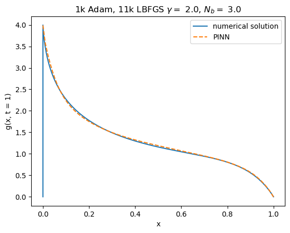
We'll check our trained solution at \(t = 1\) against a numerical solver, specifically the solver included in the dadi package. dadi works in the untransformed frequency \(\phi(x,t)\), so we'll need to multiply it by \(x(1-x)\) to convert it to \(g(x,t)\)

import dadi

TEST_GAMMA = 2.0
TEST_IC = initial_g(XS, TEST_GAMMA)
TEST_NS = 3.0
TEST_NVALS = NFUNC(TS, TEST_NS)


def calc_dadi(tf=1.0, pts=300):
    xx = dadi.Numerics.default_grid(pts=pts)
    phi0 = dadi.PhiManip.phi_1D(xx, gamma=TEST_GAMMA)
    phif = dadi.Integration.one_pop(phi0, xx, tf, lambda t: NFUNC(t, TEST_NS), gamma=TEST_GAMMA)
    return xx, phif, phi0

x_dadi, phi_dadi, phi0_dadi = calc_dadi()
x_test = jnp.linspace(0, 1, 100)
g_test = jax.vmap(model, in_axes=(0, None, None))(x_test, 1.0, (TEST_NVALS, TEST_IC))

# plt.figure(figsize=(5, 4))
plt.plot(x_dadi, phi_dadi * x_dadi * (1.0 - x_dadi), label="numerical solution")  # convert phi to g
plt.plot(x_test, g_test, label="PINN", ls="--")
plt.legend()
plt.xlabel("x")
plt.ylabel("g(x, t = 1)")
# plt.tight_layout()
plt.title(rf"1k Adam, 11k LBFGS $\gamma =$ {TEST_GAMMA}, $N_b =$ {TEST_NS}")

Text(0.5, 1.0, '1k Adam, 11k LBFGS $\\gamma =$ 2.0, $N_b =$ 3.0')