PINN¤
The PDE our PINN will be learning is the diffusion approximation to the Wright-Fisher model of the single-locus allele frequency spectrum \(\phi(x, t)\) from population genetics. We will consider genetic drift, selection, and mutation, but not migration:
the first term accounts for drift, the second term selection, \(N(t)\) is the relative population size, and \(\gamma\) is the population-scaled selection coefficient. We are working in the rescaled density \(g(x,t) = x(1-x)\phi(x,t)\), which transforms the singular boundary behaviour at \(x = 0\) into a finite value (i.e. a Dirichlet boundary condition).
The boundary conditions are
where \(\theta\) is the population-scaled mutation rate, and
The initial condition is $$ g(x, t = 0) = \theta N_0 \frac{1 - e^{-2\gamma(1-x)}}{1 - e^{-2\gamma}}. $$
For this example, we'll fix \(\gamma = 1\) and define \(N(t) = 2t + 1\), so that \(N(0) = 1\).
import jax

jax.config.update("jax_enable_x64", True)  # PINNs generally need float64
import equinox as eqx
import jax.numpy as jnp
import jax.random as jr
import matplotlib.pyplot as plt
from jaxtyping import Array

from popinn import (
    PINN,
    AdamConfig,
    LBFGSConfig,
    Loss,
    ResidualTerm,
    plot_training_history,
    train_model,
)
# Fixed values


THETA = 1.0  # population-scaled mutation rate
GAMMA = 1.0  # population-scaled selection coefficient
NFUNC = lambda t: 2.0 * t + 1  # linear population size increase

# x-coordinate boundaries
XMIN = 0.0
XMAX = 1.0

# t-coordinate maximum
TMAX = 1.0

# colocation grid lengths
NUM_PDE_PTS = 100  # points per spatial/temporal coordinate axis on PDE interior
NUM_EDGE_PTS = 256  # points used to sample the IC/boundary coordinate lines
Residual Terms¤
First we'll define the per-point residual functions, one for each of our equations listed above.
Important syntax note
Residual functions are factories that must follow the signature:
so that they can be used by the grid evaluation methods used inResidualTerm and Loss. In this example, we have no auxiliary inputs, but we still need to include aux as an argument in the inner function.
# PDE residual
def pde_residual(model):
    def r(x, t, aux):

        dg_dx = model.D(0)(x, t)  # d/dx
        dg_dt = model.D(1)(x, t)  # d/dt
        d2g_dx2 = model.D(0, 0)(x, t)  # d2/dx2

        diff = x * (1.0 - x) / (2.0 * NFUNC(t)) * d2g_dx2  # diffusion
        sel = GAMMA * x * (1.0 - x) * dg_dx  # selection

        # we weight the per-point residuals by their frequency x, as the gradients
        # tend to be very large at low-frequency. Wrapping x in
        # jax.lax.stop_gradient treats it like a constant, rather than a differentiable
        # quantity, so it doesn't change the PDE we are trying to solve
        return (dg_dt + sel - diff) * jax.lax.stop_gradient(x)

    return r
# Left BC residual
def left_bc_residual(model):
    def r(x, t, aux):
        return model(x, t) - THETA * NFUNC(t)

    return r
def initial_g(x, _gamma):
    return NFUNC(0) * THETA * jnp.expm1(-2.0 * _gamma * (1 - x)) / jnp.expm1(-2.0 * _gamma)


# initial condition residual
def ic_residual(model):
    def r(x, t, aux):
        return model(x, t) - initial_g(x, GAMMA)

    return r
Now that we've defined our per-point residual functions, we can turn each into a ResidualTerm and pass them to Loss to build the total loss. By default, each term has a weight of 1. We can define custom weights for each term using a mapping or a subclass of AbstractWeights like FixedWeights, but for this example we'll stick with the default.
total_loss = Loss(
    [
        ResidualTerm(name="pde", residual_fn=pde_residual),
        ResidualTerm(name="left_bc", residual_fn=left_bc_residual),
        ResidualTerm(name="right_bc", residual_fn=right_bc_residual),
        ResidualTerm(name="ic", residual_fn=ic_residual),
    ]
)
Training Data¤
Next, we set up a data container with equinox.Module. Each field of the container should be called <name>_coords, where <name> corresponds to the name of a ResidualTerm defined above. The only field that can be something other than <name>_coords is aux, which is a tuple containing all the auxiliary inputs for our model. Since we have no auxiliary inputs, we must pass an empty tuple to aux.
Important syntax note
Reiterating because this is important: the data containers must follow the format
class TrainingData(eqx.Module):
    <name1>_coords: tuple[Array]
    <name2>_coords: tuple[Array]
    # ...
    aux: tuple
<name#> corresponds to the name of each defined ResidualTerm. Ex: pde_coords for the ResidualTerm named 'pde' above.
Why equinox.Module and not a dictionary?
The short answer is that it's what Loss expects: it reads the data like data.pde_coords, not data['pde_coords'], so just passing in a dictionary will fail. The longer answer is that an equinox.Module gives us a few perks a dictionary wouldn't. Its fields are immutable, so we can't accidentally modify the data in place; instead, Equinox defines a clean interface for updating pytrees (see JAX's documentation to learn more about pytrees) with equinox.tree_at, which matters once we want to, say, resample the collocation data each training step. Finally, it keeps everything consistent across popinn: anything that passes through jit/grad is an equinox.Module.
class TrainingData(eqx.Module):
    pde_coords: tuple[Array]
    ic_coords: tuple[Array]
    left_bc_coords: tuple[Array]
    right_bc_coords: tuple[Array]
    aux: tuple


X_pde = jnp.linspace(XMIN, XMAX, NUM_PDE_PTS)
T_pde = jnp.linspace(0, TMAX, NUM_PDE_PTS)

X_ic = jnp.linspace(XMIN, XMAX, NUM_EDGE_PTS)
T_ic = jnp.zeros(1)

T_bc = jnp.linspace(0, TMAX, NUM_EDGE_PTS)
X_lbc = XMIN * jnp.ones(1)
X_rbc = XMAX * jnp.ones(1)


data = TrainingData(
    pde_coords=(X_pde, T_pde),
    ic_coords=(X_ic, T_ic),
    left_bc_coords=(X_lbc, T_bc),
    right_bc_coords=(X_rbc, T_bc),
    aux=(),
)
Tuples and coordinate axis mapping
By passing in the coordinates as a tuple of arrays, rather than a stacked jax.numpy array, we can have coordinates arrays with different lengths. Notice how, for example, T_ic is an array with shape (1,) while X_ic has a shape (NUM_EDGE_PTS,).
Under the hood, ResidualTerm will evaluate its corresponding function over a cartesian-product of each coordinate axis using jax.vmap. This means we never need to construct a meshgrid of data ourselves and a large array with shape (NUM_PDE_PTS, NUM_PDE_PTS) is only materialized in memory when the loss is computed. This isn't a concern in a this small example, but can be in problems with higher numbers of dimensions or with additional auxiliary inputs.
Initialize Model and Train¤
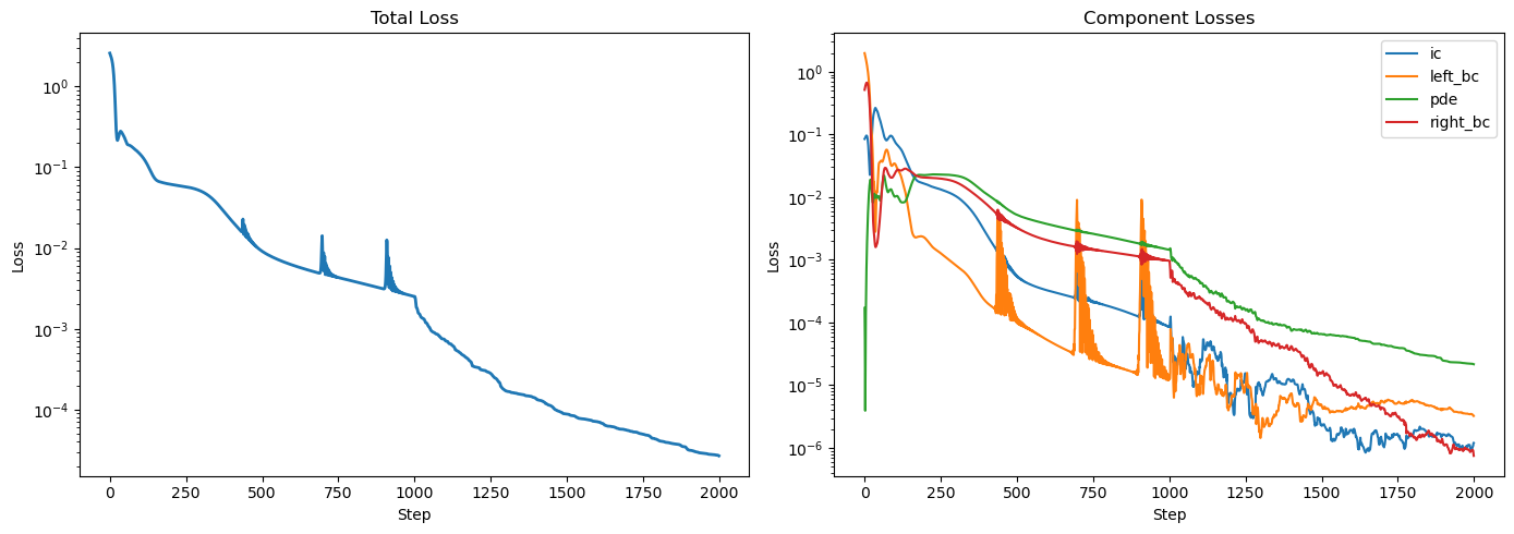
We'll first train with 500 Adam steps, then 1k of L-BFGS:
key = jr.PRNGKey(3)
model = PINN(key, num_coords=2)  # our coordinates are x & t

model, history = train_model(
    model,
    data,
    total_loss,
    [AdamConfig(log_every=100, num_epochs=1000, lr=1e-3), LBFGSConfig(log_every=100, num_epochs=1000)],
)
[Adam] Starting (1000 epochs)
[Adam] Epoch      1 | total: 2.58e+00 | ic: 8.49e-02  left_bc: 1.98e+00  pde: 1.71e-04  right_bc: 5.16e-01
[Adam] Epoch    100 | total: 1.46e-01 | ic: 7.77e-02  left_bc: 3.43e-02  pde: 1.02e-02  right_bc: 2.37e-02
[Adam] Epoch    200 | total: 6.15e-02 | ic: 1.63e-02  left_bc: 2.21e-03  pde: 2.25e-02  right_bc: 2.05e-02
[Adam] Epoch    300 | total: 5.07e-02 | ic: 1.04e-02  left_bc: 8.21e-04  pde: 2.21e-02  right_bc: 1.74e-02
[Adam] Epoch    400 | total: 2.20e-02 | ic: 2.62e-03  left_bc: 2.13e-04  pde: 1.14e-02  right_bc: 7.82e-03
[Adam] Epoch    500 | total: 9.19e-03 | ic: 5.44e-04  left_bc: 9.94e-05  pde: 5.25e-03  right_bc: 3.30e-03
[Adam] Epoch    600 | total: 6.16e-03 | ic: 3.26e-04  left_bc: 5.30e-05  pde: 3.73e-03  right_bc: 2.05e-03
[Adam] Epoch    700 | total: 5.33e-03 | ic: 2.32e-04  left_bc: 6.49e-04  pde: 2.96e-03  right_bc: 1.49e-03
[Adam] Epoch    800 | total: 3.89e-03 | ic: 1.83e-04  left_bc: 2.10e-05  pde: 2.33e-03  right_bc: 1.35e-03
[Adam] Epoch    900 | total: 3.12e-03 | ic: 1.27e-04  left_bc: 3.02e-05  pde: 1.83e-03  right_bc: 1.13e-03
[Adam] Epoch   1000 | total: 2.52e-03 | ic: 8.54e-05  left_bc: 1.42e-05  pde: 1.45e-03  right_bc: 9.65e-04
[L-BFGS] Starting (1000 max iterations)
[L-BFGS] Step      1 | total: 2.51e-03 | ic: 8.50e-05  left_bc: 1.29e-05  pde: 1.45e-03  right_bc: 9.65e-04
[L-BFGS] Step    100 | total: 7.33e-04 | ic: 1.96e-05  left_bc: 7.00e-06  pde: 4.57e-04  right_bc: 2.50e-04
[L-BFGS] Step    200 | total: 3.37e-04 | ic: 7.49e-06  left_bc: 4.56e-06  pde: 2.09e-04  right_bc: 1.16e-04
[L-BFGS] Step    300 | total: 1.71e-04 | ic: 9.37e-06  left_bc: 1.44e-06  pde: 1.10e-04  right_bc: 5.08e-05
[L-BFGS] Step    400 | total: 1.37e-04 | ic: 1.15e-05  left_bc: 7.36e-06  pde: 7.68e-05  right_bc: 4.11e-05
[L-BFGS] Step    500 | total: 8.83e-05 | ic: 2.33e-06  left_bc: 4.88e-06  pde: 6.57e-05  right_bc: 1.54e-05
[L-BFGS] Step    600 | total: 7.10e-05 | ic: 1.92e-06  left_bc: 4.48e-06  pde: 5.76e-05  right_bc: 7.09e-06
[L-BFGS] Step    700 | total: 5.54e-05 | ic: 1.24e-06  left_bc: 5.57e-06  pde: 4.42e-05  right_bc: 4.34e-06
[L-BFGS] Step    800 | total: 4.20e-05 | ic: 1.58e-06  left_bc: 5.68e-06  pde: 3.32e-05  right_bc: 1.55e-06
[L-BFGS] Step    900 | total: 3.16e-05 | ic: 1.62e-06  left_bc: 4.15e-06  pde: 2.47e-05  right_bc: 1.18e-06
[L-BFGS] Step   1000 | total: 2.68e-05 | ic: 1.20e-06  left_bc: 3.24e-06  pde: 2.16e-05  right_bc: 7.48e-07
We'll check our trained solution at \(t = 1\) against a numerical solver, specifically the solver included in the dadi package. dadi works in the untransformed frequency \(\phi(x,t)\), so we'll need to multiply it by \(x(1-x)\) to convert it to \(g(x,t)\)
import dadi


def calc_dadi(tf=1.0, pts=300):
    xx = dadi.Numerics.default_grid(pts=pts)
    phi0 = dadi.PhiManip.phi_1D(xx, gamma=GAMMA)
    phif = dadi.Integration.one_pop(phi0, xx, tf, lambda t: NFUNC(t), gamma=GAMMA)
    return xx, phif, phi0
plt.figure(figsize=(5, 4))
plt.plot(x_dadi, phi_dadi * x_dadi * (1.0 - x_dadi), label="numerical solution")  # convert phi to g
plt.plot(X_pde, g_test, label="PINN", ls="--")
plt.legend()
plt.xlabel("x")
plt.ylabel("g(x, t = 1)")
plt.tight_layout()
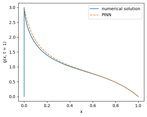
The PINN tracks the solution well. We can improve the solution recovery at low frequency by traning for longer or by including more collocation points in that region and re-trainig. We could also try retraining with a larger weight for the PDE loss term or increasing the size of our network. Like most neural networks, PINNs typically require some fine-tuning.
Next Steps¤
Review the core principles section, then move on to the P\(^2\)INN example to see auxiliary inputs in action.